Conditional generators are most useful for conditions nobody has observed, and that is exactly where FID or KID cannot be computed, because they need real samples of the target. We score each generated sample using only the training distribution: a global realism term plus an attribute-by-attribute faithfulness term. The score filters, ranks, and can even reject samples before they are decoded; on CelebA and RxRx1 the samples it keeps improve ΔKID by 39–44% over random subsets of the same size.
Evaluating what has never been measured
Conditional diffusion models can generate images for a requested condition: a tuple of attributes, or a biological perturbation applied to a given cell type. In science, the appeal is the conditions nobody has measured yet. A generator that simulates perturbations in silico could help decide which ones to test in the wet lab first.
That only helps if we can tell which generated samples to believe, and here evaluation runs into a circularity. FID, KID, and their conditional variants compare generated samples with real samples from the target distribution, and in the extrapolative regime that distribution is unavailable by definition. These metrics remain useful in benchmarks where we deliberately hold real data out, but they cannot decide whether one particular sample should be trusted at deployment time.
So we asked a different question: what information about sample quality is identifiable from the real training distribution alone?
What the training data can and cannot tell us
Part of the answer is negative. If a combination of attributes never appears in the real data, nothing in the data says what its images should look like, unless we assume how it relates to the combinations we did see. No score built from the training data alone can certify that a sample of an unseen combination is fully right.
What survives is a check one attribute at a time: does the sample look more like the requested value of each attribute than like the alternatives? CelebA makes this concrete. Four binary attributes (male, smiling, blond hair, eyeglasses) give 16 combinations, and we train on only five of them: 0000 and the four that switch on a single attribute, 1000, 0100, 0010 and 0001. Every attribute has then been seen changing on its own, so its effect can be read off the data, and a sample of any of the 16 combinations can be checked attribute by attribute.
Without that kind of coverage, the evidence becomes ambiguous. Had training seen only 0000 and 1111, the data would show that the images change, but not which attribute is responsible. For four binary attributes, five is the smallest number of observed combinations that avoids this; the star around 0000 is one layout that reaches it, not the only one.
Two things we can still check
Two quantities stay observable, and they catch two different failures: a sample can be realistic but wrong for the requested condition, or it can express the condition while falling outside the manifold of real data. Existing post-hoc tools usually see one side. Out-of-distribution scores measure global compatibility with real data, and prompt- or classifier-based scores measure agreement with a condition. We combine both in the feature space of a pretrained extractor \(\Phi\), using only the generated sample and statistics of real training features.
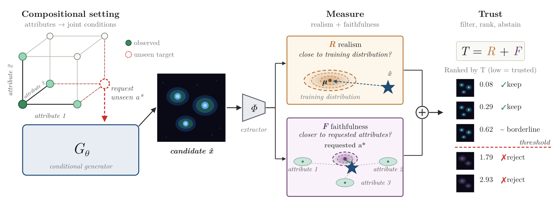
Realism \(R\) asks how typical the sample's features \(y\) are of real data: it is a distance to the real feature distribution that accounts for how features vary and correlate. Faithfulness \(F\) carries out the attribute-by-attribute check. For each value \(v\) of attribute \(k\), the real samples with that value define a prototype, and \(d_k(y; v)\) measures how far the sample is from it. For the requested value \(t\), the margin
is negative when the sample is closer to \(t\) than to every alternative. Averaging the margins over attributes gives \(F\), and the trust score is \(T = R + F\), with lower meaning more trusted. \(R\) catches samples that are far from anything real; \(F\) catches samples that look real but show the wrong attributes.
Request a condition
columns: cell type · rows: perturbation
Shaded cells were observed in training. Every value of each attribute appears with the reference value (c1 or p1) of the other, but the “?” combinations never do.
Generated samples
- real training data
- kept
- rejected
- malformed sample
- requested target
The score is only as good as the geometry of \(\Phi\). In OpenPhenom's feature space it fails: mean trust barely tracks sample quality, because its features barely vary within a class, and distances that scale each direction by that variation end up amplifying noise.
Does it pick better samples?
Besides CelebA, we test on RxRx1, a fluorescence microscopy dataset whose attributes are cell type and siRNA perturbation, with some combinations held out of training. On both we train a vanilla conditional diffusion model and two REPA variants, aligned to DINOv3 or SigLIP. A generated sample is accepted if its trust score is below the 95th percentile of real samples' scores, and the accepted set is compared with a random subset of the same size, using KID against held-out real samples that the score never sees.
| Dataset · model | Accept% | ΔKIDtrust | ΔKIDrandom | Δ% | ρ(T) |
|---|---|---|---|---|---|
| CelebA · Vanilla | 58.7 | 0.224 ± .009 | 0.368 ± .020 | +39.1 | 0.96 |
| CelebA · REPA (DINOv3) | 55.4 | 0.228 ± .010 | 0.401 ± .031 | +43.1 | 0.96 |
| CelebA · REPA (SigLIP) | 56.1 | 0.239 ± .018 | 0.423 ± .020 | +43.6 | 0.96 |
| RxRx1 · Vanilla | 4.4 | 0.196 ± .006 | 0.323 ± .013 | +39.4 | 0.90 |
| RxRx1 · REPA (DINOv3) | 5.5 | 0.197 ± .006 | 0.333 ± .019 | +40.8 | 0.90 |
| RxRx1 · REPA (SigLIP) | 6.1 | 0.181 ± .003 | 0.312 ± .019 | +42.0 | 0.87 |
On both datasets the trusted samples are clearly closer to the real target than random ones, even though on RxRx1 the threshold keeps only a small fraction of generations. A condition's mean trust also tracks how hard that condition is.
Biology, measured independently
DINOv3 is a learned encoder, so we also checked the selection in CellProfiler space, a set of interpretable morphology measurements computed directly from segmented cells. In every setting, trusted samples are morphologically closer to real cells of their condition than random ones, on seen and unseen conditions alike, although unseen conditions stay further from real morphology.
Abstaining before the image exists
Scoring after generation means paying for the full denoising run first. Because the score lives in a fixed real-data geometry, we can instead evaluate it on the generator's internal representations, mapped into the feature space of \(\Phi\) by a small translator trained to preserve that geometry.
Preserving the geometry is what matters. REPA-trained generators already align their internal features with a pretrained encoder, but on RxRx1, scoring those features directly picks worse samples than chance, because the alignment does not keep the covariance structure the score relies on. With the translator, filtering works from inside the generator, and it works early: partway through denoising the score already picks out better samples, so rejected ones never cost the rest of the compute.
What is still open
The theory covers discrete attributes; continuous conditioning variables and weaker identifiability conditions remain open. And today the score only rejects poor samples. A natural next step is to use it to steer generation toward high-trust regions.
Technical details
The score in full
We work with normalized features \(y(x) = \Phi(x) / \lVert \Phi(x) \rVert_2\) and fit every mean, covariance, precision matrix, and calibration constant on normalized real training features. With \(\mu_{\text{real}}\) and \(\Sigma_{\text{real}}\) the mean and regularized covariance of the real features,
and \(R(y) = (E_{\text{real}}(y) - m_R) / s_R\), where \(m_R\) and \(s_R\) are the mean and standard deviation of \(E_{\text{real}}\) on real calibration features. For faithfulness, the prototype \(\eta_{k,v} = \mathbb{E}[\,y \mid a_k = v\,]\) averages the real features with value \(v\), \(P_k \succ 0\) is a shared precision matrix estimated from the pooled within-value covariance, and
Each margin is standardized on real samples that carry the requested value, \(F_k(y;t) = (M_k(y;t) - m_{k,t}) / s_{k,t}\), and
Identifiability, formally
Without assumptions relating observed and unobserved conditions, the conditional feature distribution at a missing condition \(a^\star\) is not identifiable (Proposition 1). The CelebA design is an instance of reference coverage: writing \(a_{-k}\) for all attributes except \(a_k\), there is a reference condition \(\bar a\) such that, for every attribute \(k\) and every value \(v \in \mathcal{A}_k\),
Under it, the reference prototypes \(\mu^{\text{ref}}_{k,v} = \mathbb{E}[\,y \mid a_k = v,\ a_{-k} = \bar a_{-k}\,]\) and the margins built from them are point-identified from the observed data (Proposition 2). Any support that identifies every attribute-value effect without structural assumptions needs at least \(1 + \sum_k (|\mathcal{A}_k| - 1)\) observed conditions, which reference coverage attains (Proposition 3). The implemented score uses the pooled \(\eta_{k,v}\) instead, which is more sample-efficient. The appendix gives sufficient conditions under which the pooled comparator makes the same attribute-wise decisions as the anchored one, and measures their agreement: 0.990 to 1.000 across CelebA attributes, 0.997 for RxRx1 cell type, and 0.803 for the finer-grained RxRx1 siRNA attribute.
Validation and alternative scorers
KID uses the held-out real target samples as ground truth: \(\Delta\text{KID} = \text{KID}(\text{gen}, \text{real}_A) - \text{KID}(\text{real}_B, \text{real}_A)\), always in a fixed DINOv3 feature space. In an appendix ablation, alternative scorers in the same feature space (a per-attribute linear probe, a per-attribute nearest-neighbour distance, and CLIP alignment on CelebA) all produce near-degenerate real-data thresholds that accept almost every sample. Only the calibrated Mahalanobis score gave both a usable acceptance rate and a substantial KID improvement.
Ranking by trust decile
We split generated samples into class-balanced trust deciles, train a condition classifier on each decile separately, and evaluate it on held-out real data.
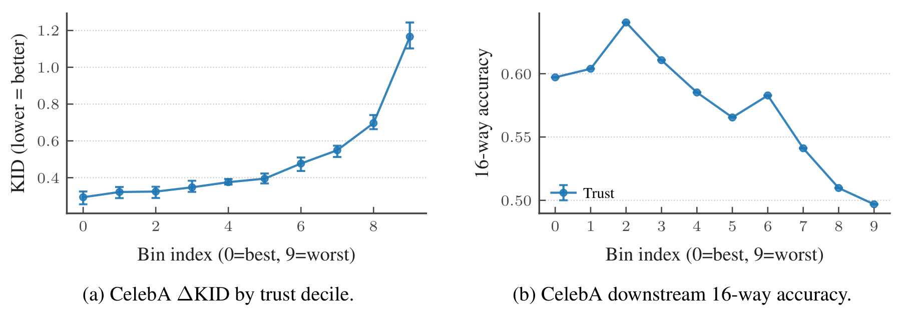
On CelebA, ΔKID degrades roughly fourfold from the best to the worst decile, and downstream accuracy drops by about 10% when training on the least trusted samples. RxRx1 shows the same ordering for KID and downstream classification, and in CellProfiler space more trusted deciles train better cell-type and condition classifiers.
CellProfiler morphology
Each generated cell's distance to the centroid of the matching real condition is standardized by the spread between random halves of the real data, so 0 is typical real-to-real variation and anything above is excess deviation. All six reductions have bootstrap confidence intervals strictly below zero. The per-feature breakdown points to biologically meaningful axes: per-cell texture autocorrelation, image-level granularity, total cell-segmentation area, and cytoplasm shape regularity.
| Model · split | Accept% | z̄trust | z̄random | Δ% |
|---|---|---|---|---|
| Vanilla · seen | 66.3 | 0.055 | 0.111 | +50 |
| Vanilla · unseen | 21.9 | 0.583 | 0.712 | +18 |
| REPA (DINOv3) · seen | 61.2 | 0.024 | 0.137 | +83 |
| REPA (DINOv3) · unseen | 21.0 | 0.535 | 0.755 | +29 |
| REPA (SigLIP) · seen | 65.7 | 0.032 | 0.126 | +75 |
| REPA (SigLIP) · unseen | 23.5 | 0.827 | 1.020 | +19 |
Scoring during generation
A shallow MLP translator \(g_{\phi,\ell}\) maps the representation at layer \(\ell\) and denoising step \(\tau\) into the \(\Phi\) feature space. At inference time we evaluate the same \(T\) on the mapped feature and abstain as soon as \(T(y^{\text{map}}_{\ell,\tau}; a^\star) > \kappa_{\ell,\tau}\) for a layer- and step-specific threshold. The REPA baseline partly works on CelebA (ρ(T) = 0.95, +31% ΔKID). With the translator on CelebA, around step 166 of 250 the filter matches the post-generation result while still saving 34% of the denoising compute.
| Features · model | Accept% | ΔKIDtrust | ΔKIDrandom | Δ% | ρ(T) |
|---|---|---|---|---|---|
| REPA · REPA (DINOv3) | 1.4 | 0.537 ± .032 | 0.329 ± .037 | −63.4 | 0.09 |
| REPA · REPA (SigLIP) | 3.9 | 0.564 ± .022 | 0.293 ± .023 | −92.3 | 0.13 |
| translator · Vanilla | 38.4 | 0.260 ± .003 | 0.346 ± .016 | +24.9 | 0.78 |
| translator · REPA (DINOv3) | 62.3 | 0.246 ± .003 | 0.372 ± .037 | +33.8 | 0.88 |
| translator · REPA (SigLIP) | 60.5 | 0.235 ± .011 | 0.329 ± .018 | +28.7 | 0.70 |
Citation
@inproceedings{demirel2026assessing,
  title={Assessing Sample Quality in Conditional Generation under Compositional Shift},
  author={Berker Demirel and Valentino Maiorca and Marco Fumero and Theofanis Karaletsos and Francesco Locatello},
  booktitle={The Fortieth Annual Conference on Neural Information Processing Systems},
  year={2026},
  url={https://arxiv.org/abs/2606.09601}
}